Executive Summary
A 2026 Applied Ocean Research study revisits how extreme sea levels are estimated for offshore design. We unpack what the design codes actually demand of a still-water-level figure, where the survey and metocean leads carry the exposure, and the datum, record-length and non-stationarity traps that quietly corrupt a return-level estimate. The article closes with concrete validation steps before any design level enters the basis of design.
On this page5 sections
What the study puts back on the table
A recent paper in Applied Ocean Research (Volume 175, October 2026) by Jie Hu, Yibin Liu, Adrian C.H. Lai and Joseph H.W. Lee returns to a question that sits under almost every fixed-structure design basis: how do we estimate an extreme sea level with enough confidence to set a deck elevation, an air gap, or a coastal defence crest. The full text was not available to us at the time of writing, so we will not attribute specific methods or results to the authors. What the publication does confirm is that extreme sea level estimation remains an open methodological problem worth a journal treatment in 2026 – not a settled procedure that a metocean lead can accept from a data provider without scrutiny.
That is the useful signal. Extreme sea level is one of the few metocean parameters where the estimation method, the input record and the vertical datum each carry error that can move the design number by tenths of a metre, and where tenths of a metre decide whether a wave crest clears the underside of a topside or slams into it. We use this paper as the prompt to set out what survey and metocean leads should be validating, and against which standards.
What the design codes actually demand of a still-water-level figure
Extreme sea level is not a single measurement. It is a composite of mean sea level and its trend, the astronomical tide, the meteorological surge residual, and – at the coast – wave setup and runup. Vertical land motion sits underneath all of it. The design codes treat these components explicitly.
ISO 19901-1, the metocean standard for offshore structures, requires the metocean design basis to define extreme still water level as a combination of tide, surge and long-term sea level change, referenced to a stated vertical datum, at a specified return period. DNV-RP-C205 (Environmental conditions and environmental loads) sets out the same decomposition and the extreme value machinery behind it. For fixed offshore structures the ultimate limit state is commonly tied to the 100-year return period, while abnormal-level and robustness checks under ISO 19902 reach to the 10,000-year event. Offshore wind under IEC 61400-3-1 typically works to a 50-year recurrence for many environmental parameters. Coastal and nuclear work reaches further still.
The air gap is where the still-water-level figure becomes a consequence rather than a number. ISO 19901-1 defines air gap as the clearance between the extreme still water level and the underside of the lowest exposed deck, and it must remain positive after adding the extreme wave and current crest elevation and an allowance for settlement and sea level rise. A negative air gap means wave-in-deck loading, which is a step change in global and local action, not a marginal increase. This is the reason a metocean lead cannot treat the extreme sea level as a soft input. It propagates directly into structural safety through the crest elevation and the deck clearance.
Two extreme value approaches dominate practice, and the codes recognise both:
- Direct extreme value analysis of the total still-water-level time series – either annual maxima fitted to a Generalised Extreme Value distribution, or peaks-over-threshold fitted to a Generalised Pareto distribution.
- Joint probability methods, which treat the deterministic tide and the stochastic surge separately and combine them by convolution. The skew-surge joint probability method, adopted in UK coastal flood boundary work, is the mature form because skew surge is largely independent of tidal phase and so behaves better statistically than the instantaneous non-tidal residual.
Neither is automatically correct. The choice depends on record length, on the strength of tide–surge interaction at the site, and on the return period being extrapolated to.
Where the numbers meet the datum: the survey lead’s exposure
The metocean statistician owns the distribution. The survey lead owns the vertical reference frame, and an error there is a systematic bias that no amount of statistical rigour will remove.
A tide gauge measures water level against its own gauge zero. That zero must be connected, by levelling to a stable benchmark, to the national vertical datum, and then related to the ellipsoid through a geoid model before it can be compared with GNSS-derived heights on the structure. Each link in that chain carries error. A wrongly reconciled gauge datum, or a benchmark that has itself moved, feeds a constant offset into the extreme still water level and therefore into the air gap. We have seen this class of problem treated as trivial precisely because it produces no scatter – a pure bias hides inside a clean-looking dataset.
Vertical land motion is the second survey-owned term. Subsidence at a gauge, from tectonics, glacial isostatic adjustment or local extraction, contaminates the sea level trend embedded in the record and misstates the true relative sea level at the structure over its design life. The correct treatment separates absolute sea level change from land movement using co-located continuous GNSS, CORS ties and, where available, InSAR. The same discipline that governs positioning integrity offshore applies to the vertical frame here; the reasoning we set out on what genuine rigour means for offshore positioning QA transfers directly to establishing a defensible datum for a design level.
IHO S-44 governs the hydrographic side of this – sounding datum definition, uncertainty budgeting and the separation between chart datum, lowest astronomical tide and mean sea level. A metocean design basis that quotes an extreme level without stating the datum, the epoch and the geoid model is incomplete, and any reviewer should reject it on that basis alone. The datum statement is not paperwork. It is the definition of what the number means.
The traps that turn a defensible extreme into a wrong one
Record length against return period. Extrapolating a 100-year level from twenty or thirty years of gauge data is standard, and it is where most of the uncertainty lives. The Generalised Pareto shape parameter that controls the tail is poorly constrained by short records; small changes in it swing the 1,000-year and 10,000-year levels substantially. A single point estimate quoted without a confidence interval is a red flag. Profile-likelihood or bootstrap intervals should accompany every return level, and the design team needs to see the width of that interval before deciding how much conservatism to add.
Threshold and declustering in peaks-over-threshold. The threshold choice is a genuine trade-off. Set it too low and non-extreme events bias the fit; set it too high and the sample collapses and the shape parameter becomes unstable. Threshold selection should be justified with a mean residual life plot and a demonstration that the shape parameter is stable across a range of thresholds, not fixed by convenience. Declustering matters just as much – successive peaks within one storm are not independent, and a minimum event separation of the order of days is needed to recover statistically independent extremes. Under-declustering inflates the effective sample and understates uncertainty.
Tide–surge interaction. In shallow water the surge is not independent of the tide. The largest surges often develop on the rising tide rather than at high water, which reduces the probability that the surge peak coincides with the tidal peak. Naively adding an extreme tide to an extreme surge overstates the combined level. This is exactly why skew-surge joint probability methods exist, and why the interaction has to be characterised at the specific site rather than assumed away.
Non-stationarity. Classical extreme value analysis assumes a stationary process. Sea level rise breaks that assumption over a design life of decades. A stationary fit to a record that already contains a trend will misplace the return level, and it says nothing about the level at the end of design life. The design basis must state the sea level rise allowance explicitly, tied to a named scenario and time horizon – IPCC AR6 projections are the current reference point – and the metocean lead should show the extreme level both at commissioning and at end of life. Treating a single stationary number as valid for forty years is one of the most common errors we encounter in review.
Undetected datum jumps in the record. A gauge that was re-levelled, relocated or had its zero redefined mid-record introduces a step that no distribution fit will flag. It simply corrupts the extremes. The record must be inspected for datum continuity before any analysis, and any discontinuity reconciled against the levelling history. This is a data-quality task that sits ahead of the statistics, and skipping it invalidates everything downstream.
What to validate before the design level enters the basis of design
The following are the checks we would require before signing an extreme sea level into a basis of design. Each is testable by the survey or metocean lead against a written record.
- Confirm the vertical datum chain end to end. Gauge zero to benchmark to national datum to ellipsoid, with the geoid model named and the epoch stated. Require the levelling history and the last benchmark stability check. Reject any figure quoted without an explicit datum and epoch.
- Separate absolute sea level change from vertical land motion. Demand co-located GNSS or CORS evidence for the vertical land motion term. Where the gauge sits on ground with a subsidence history, quantify it – do not fold it into the trend.
- Audit the record for continuity before the statistics. Screen for gaps, timing errors and datum steps. A discontinuity must be reconciled and documented, not smoothed over.
- Require the extreme value method to be justified for the site. Confirm whether direct or joint probability analysis was used, and confirm that tide–surge interaction was assessed rather than assumed. In shallow, interaction-prone waters, a skew-surge joint probability treatment is the defensible default.
- Demand uncertainty, not just a return level. Every 100-, 1,000- and 10,000-year figure should carry a profile-likelihood or bootstrap confidence interval, with threshold selection supported by a mean residual life plot and shape-parameter stability, and declustering at a stated minimum event separation.
- State non-stationarity explicitly. Require the extreme level at both commissioning and end of design life, with the sea level rise allowance tied to a named IPCC AR6 scenario and horizon. A single stationary number for a multi-decade asset is not acceptable.
- Close the loop to the air gap. Confirm that the extreme still water level, the wave and current crest, settlement and the sea level rise allowance have been combined per ISO 19901-1, and that positive air gap is retained across the design life. Where the margin is thin, escalate it as a design risk rather than absorbing it silently.
The engineering point running through all of this is that an extreme sea level is a chain of custody, not a single computation. The distribution fit is visible and gets the attention. The datum, the land motion, the record continuity and the stationarity assumption are quieter, and they are where the number goes wrong. A metocean or survey lead who can defend every link in that chain – and quantify the uncertainty on each – is doing the job the design codes assume has been done. One who accepts a headline return level from a data provider without it is exposing the structure to a bias no one has measured.
Published by
Ocean & Climate Observatory
Tides, Currents, Waves & Weather Forecasting
An observatory group covering metocean data analysis, hindcast modelling, oceanographic survey planning, and environmental risk assessment for marine operations.
Read next
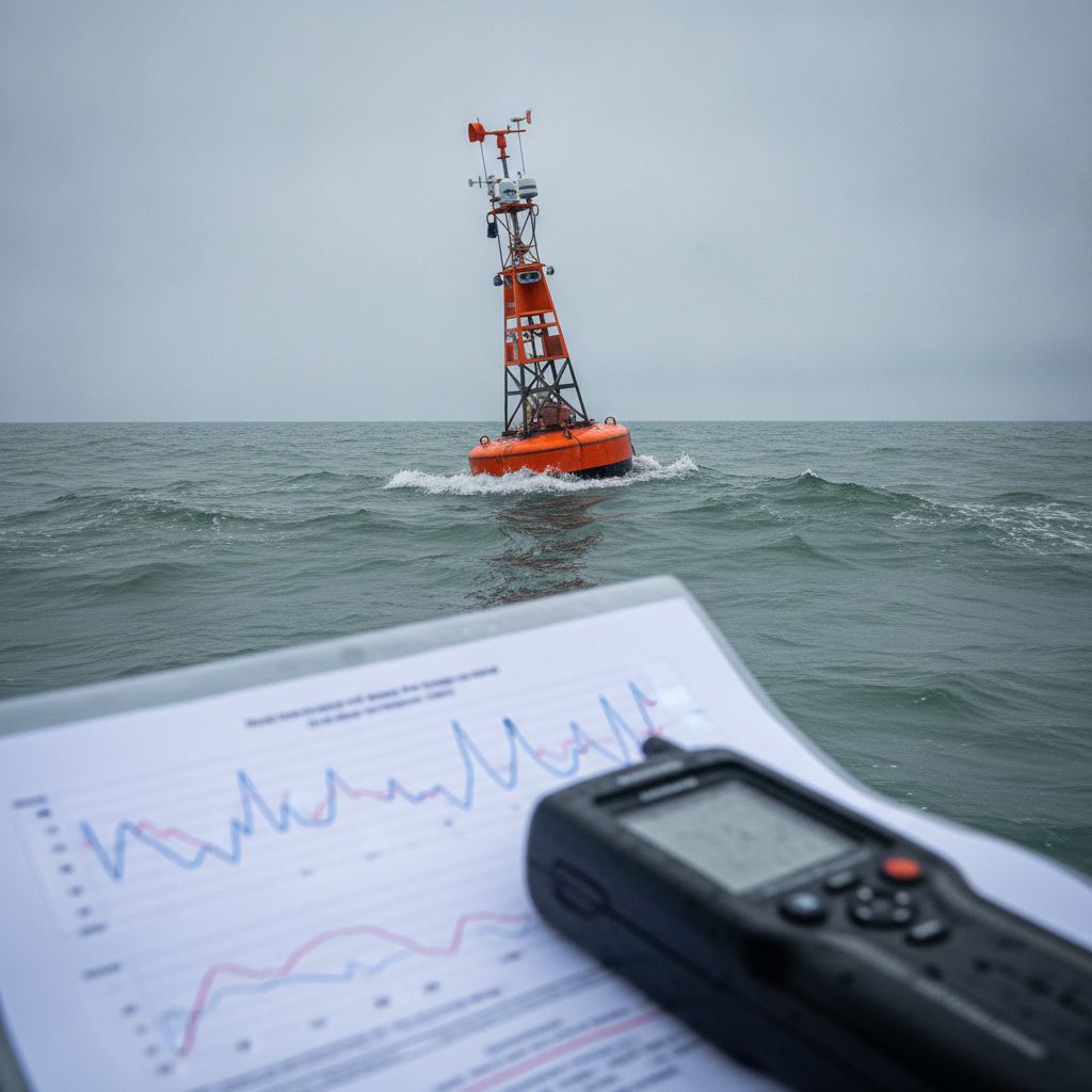
Trusting a hindcast: validating metocean models before a site campaign
Hindcast databases underpin offshore design, but model output is not truth. We unpack how to validate metocean hindcasts against in-situ data, and the standards that govern it.
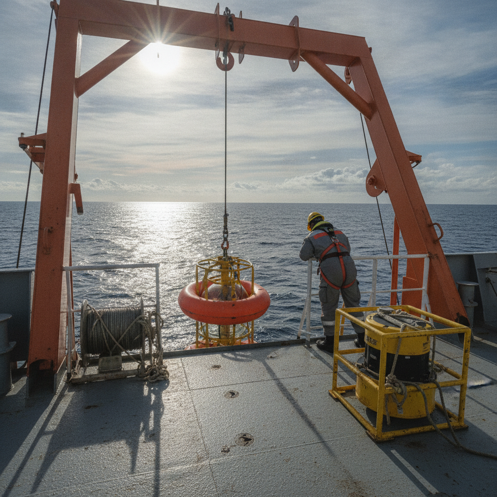
Deep-sea mining EIAs: ADCP deployment reality vs regulatory demand
Deep-sea mining EIA baseline monitoring with ADCPs: what ISA rules require for currents and sediment plumes, and where survey managers under-scope.
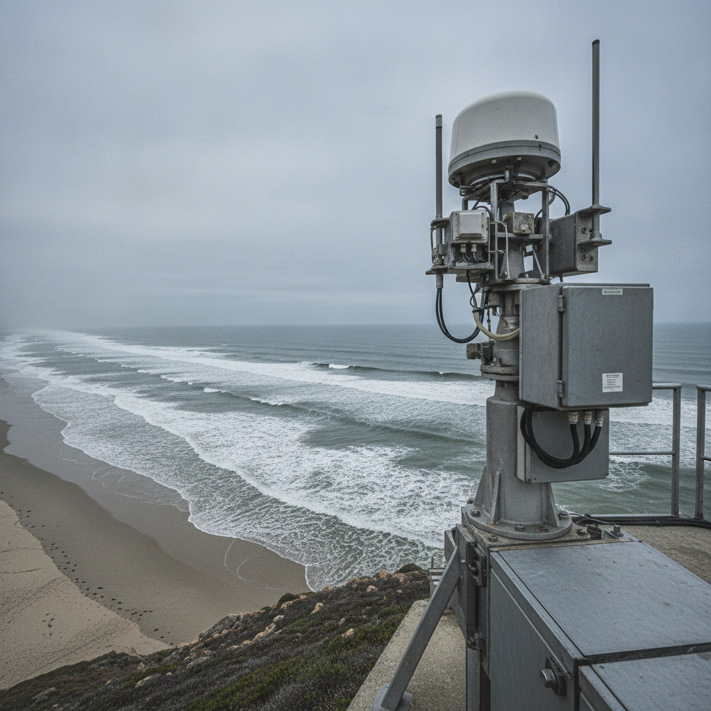
Radar-derived bathymetry: where wave inversion sits beside multibeam
How X-band radar sea-state inversion estimates depth, where it meets and misses IHO S-44, and how to blend it with multibeam for nearshore monitoring.
Offshore Geomatics Foundation Certificate · October 2026
Turn reading into certified competence
You have just read what a standard actually requires – and where it stops. The Foundation Certificate exists to prove you can work with that distinction.
Early-access list gets 40% off at launch. No spam – the waitlist is only ever used for the certificate. What the certificate covers →