Executive Summary
A recent Ocean Engineering paper proposes predicting side-scan sonar quality loss directly from AUV motion states rather than catching it in post-processing. We unpack how roll, yaw and speed variation corrupt the swath, where current QC practice and IHO S-44 leave a gap, and how to turn attitude telemetry into a defensible acceptance test. The practical prize is fewer re-runs and a motion budget written into the line plan.
On this page6 sections
The paper, and the gap it goes after
A paper in Ocean Engineering (Volume 366, Part 4), published 15 October 2026 by Zhenyu Wang, Hongsheng Lei, Hao Feng, Jianan Qiao, Yan Huang and Jiancheng Yu, addresses a problem every survey party chief already knows in their bones: AUV motion degrades side-scan sonar (SSS) imagery, and the damage is usually discovered long after the vehicle is back on deck. The contribution is to predict that quality loss from the vehicle’s own motion states rather than diagnose it visually after the fact.
The full text is not available to us, so we will not pretend to summarise its method or results. What we can do – and what a senior reader actually needs – is unpack why this framing matters, where it collides with current QC practice and hydrographic standards, and how you would fold a motion-to-quality predictor into line planning and data acceptance without over-trusting it.
This is a standards-unpacking exercise as much as a research note. The interesting question is not whether motion hurts SSS imagery (it plainly does) but what a survey standard actually requires of you, what it stays silent on, and where a predictive motion model fills that silence.
What side-scan QC standards actually pin down today
Start with what the yardsticks say. IHO S-44 (6th Edition, 2020) governs minimum standards for hydrographic surveys through order categories – Exclusive, Special, Order 1a/1b, Order 2 – expressed as total horizontal and vertical uncertainty and, for the tighter orders, feature detection. The feature-detection requirement is the one that bites SSS work: in shallow Special Order survey you are expected to detect cubic features on the order of a metre, and full seafloor search is the norm for object-detection tasks.
S-44 sets outcomes, not the ensonification geometry that delivers them. It tells you the feature you must detect and the uncertainty you must stay inside. It does not tell you the maximum roll rate your towfish or hull-mounted array may experience, nor the speed variation your along-track sampling can tolerate before a metre-cube target falls through a coverage gap. Those constraints live in method statements, client specifications and – most of the time – in the experience of the processor squinting at a waterfall display.
The rest of the QC scaffolding is procedural. IMCA and IOGP survey guidance, client route-survey specs and the surveyor’s own procedures typically demand overlap between adjacent lines sufficient to cover the nadir gap, calibrated-target confidence checks, and 100% visual inspection of the mosaic. That works, but the acceptance decision remains largely qualitative and retrospective. Motion is logged by the AUV’s inertial navigation system continuously, at high rate, and yet it is rarely tied numerically to a pass/fail on the imagery it produced. That disconnect is the gap the paper aims at.
How motion actually corrupts the swath
To judge any motion-to-quality predictor you have to be honest about the physics it is modelling. On an AUV the sonar is rigidly mounted, so the vehicle’s attitude is the array’s attitude. Every degree of freedom does something distinct to the image.
- Yaw and crab. A cross-track current sets up a crab angle between heading and course made good. The swath rotates relative to the track, features shift geometrically, and along-track energy smears because successive pings ensonify overlapping-but-offset ground. During a heading correction the yaw rate compresses one side of the swath and stretches the other.
- Roll. SSS geometry assumes a near-horizontal array. Roll tilts the vertical beam pattern, moves the peak of the ensonification lobe, shifts the effective nadir and unbalances port/starboard intensity. A few degrees is enough to visibly bias the mosaic.
- Pitch and heave. These couple straight into altitude, and altitude is the hidden variable in every slant-range-to-ground-range correction. That correction assumes a flat seafloor at constant altitude; a pitching, heaving vehicle over rugged terrain violates both assumptions and warps the geo-referenced position of every target on the line.
- Speed variation. Along-track resolution is set by the angular beamwidth times slant range, and the sampling that preserves it depends on ping rate versus ground speed. If surge variation pushes the speed over ground around, ping spacing wanders. Exceed roughly half a footprint between pings and you under-sample – a metre-cube target can sit in the gap and never register, while the coverage plot still shows green.
The important point for QC is that none of this is captured by coverage percentage alone. You can hold nominal line spacing, log 100% area coverage, and still deliver imagery that fails feature detection because the along-track sampling collapsed in a beam-on current or the roll excursions dumped the nadir. A motion-aware predictor is attractive precisely because the INS already holds every input it needs – attitude, angular rates, velocity – time-stamped ping by ping.
Turning attitude telemetry into a QC decision
The operational value shows up in two places: before the dive, in line planning, and after data-on, in triage.
In planning, a validated motion-to-quality relationship lets you convert an environmental forecast into a survey geometry. If the model says quality falls off a cliff beyond a given crab angle or yaw rate, you plan line headings to run with or against the dominant tidal or current axis rather than beam-on to it, and you schedule the exposed lines for slack water. You add run-in and run-out distances – commonly a few hundred metres before data-on – so the INS and vehicle attitude settle and no feature is acquired mid-turn. This is the same discipline that separates a clean multi-day AUV programme from one that burns endurance re-flying lines, a point we have made before in the context of planning survey work for long-endurance dives where re-runs are far more expensive than a conservative first pass.
In post-dive triage, the predictor becomes a first-pass filter. Instead of a processor scrolling every line cold, the motion record flags segments where predicted quality drops below the feature-detection threshold, and inspection effort concentrates there. On a multi-hundred-kilometre route survey that is a real saving in processor hours and in the latency between recovery and a go/no-go on re-flying. It also gives you an auditable trail: the acceptance decision references a logged motion metric, not only a signature on a visual-QC sheet.
The prerequisite that makes or breaks any of this is time synchronisation. The attitude and rate stream must be aligned to the sonar ping stream to better than a ping interval – a hardware PPS or PTP discipline, not loosely coupled system clocks. Get the timing wrong and you correlate motion with the wrong pings, and the predictor learns noise. The same navigation stack that feeds SSS geo-referencing feeds the predictor, so the integrity of the DVL-aided INS solution, and the attitude it reports, is doing double duty; the confidence you can place in a vehicle’s position and heading when acoustics are marginal is a related problem we have looked at under visual navigation as a hedge for AUV position confidence.
Where a motion predictor will mislead you
A predictive model is only as good as the assumptions baked into it, and there are several ways this class of model flatters itself.
Confounding with the seafloor. Motion tends to rise where the terrain is rugged, because the vehicle is terrain-following, and rugged terrain independently degrades imagery through layover, shadowing and grazing-angle change. A model that regresses quality on motion alone risks attributing to motion what the bottom type caused. Any credible predictor has to be conditioned on, or at least tested across, contrasting bottom types – soft mud plain versus rock and boulder fields – because target contrast and the motion tolerance are not independent.
Domain transfer. A relationship trained on one vehicle, one sonar frequency and one operating altitude will not port cleanly to another. A 400 kHz survey at 15 m altitude and a 900 kHz high-resolution pass at 8 m have different footprints, ping rates and sensitivities to the same roll excursion. Treat a transferred model as unvalidated until proven otherwise on the actual configuration.
Benign versus damaging motion. Not all attitude excursions matter equally. Slow heave that the altitude loop tracks smoothly may cost little; a sharp yaw transient at data-on may cost a target. A scalar “motion index” that does not distinguish these will both false-reject good data and false-accept bad. The QC economics of that trade-off are real – false rejects waste re-fly time, false accepts leak defects into the deliverable – and the threshold has to be set with both in view.
The green-light trap. A motion-OK flag says nothing about acoustic interference, cross-talk, nadir noise or a mis-set time-varying gain. It is a necessary condition, not a sufficient one. It cannot replace calibrated-target detection checks or full visual inspection where the specification demands them; it reorders and prioritises that work.
What to do with this now
Whether or not you adopt the specific method in the paper, the direction is sound and you can act on it with the tooling you already have.
- Log and sync the full motion state at ping resolution. Roll, pitch, heading, all three angular rates and velocity, hardware-synchronised to the sonar ping clock to better than one ping interval. Without this, no motion-to-quality analysis – theirs or yours – is trustworthy.
- Write a motion budget into the line plan, not just line spacing. Specify maximum crab angle, roll amplitude, yaw rate and speed variation tied to your sonar geometry and the S-44 order you are working to. Make it a planning parameter alongside altitude and speed.
- Plan headings against the environment. Orient lines with or against the dominant current axis rather than beam-on, sequence exposed lines to slack water, and set run-in/run-out of a few hundred metres so no feature is acquired during a turn or before attitude settles.
- Set overlap for worst-case crab, not nominal. Adjacent-line overlap should cover the nadir gap under the predicted crab and altitude excursion for that area, not under flat-calm assumptions. For object-detection tasks that usually means planning to well above 100% coverage.
- Use motion flags as triage, then validate against detection. Deploy the predictor as a first-pass filter to concentrate inspection, and prove it against calibrated targets or seeded features before you let it influence acceptance. Track false-reject and false-accept rates as QC KPIs.
- Hold the standard as the acceptance criterion. The pass/fail must remain “does the imagery meet the S-44 order’s feature-detection requirement”, with the motion metric as evidence supporting that decision and an audit trail behind it – never a substitute for it.
The value here is not a clever regression. It is closing the loop between the navigation data an AUV already produces and the QC decision a survey team currently makes by eye and after the fact. Done with discipline, it moves quality control upstream into planning and real-time triage, and it gives the client a defensible, quantitative basis for why a line passed or why it will be re-flown.
Based on: Predicting side-scan sonar quality loss from AUV motion
Published by
Hydrographic Methods Committee
Bathymetry, Multibeam & Seabed Mapping
An independent review committee focused on hydrographic survey methodology, IHO standards interpretation, and seabed mapping best practices for offshore and coastal projects.
Read next
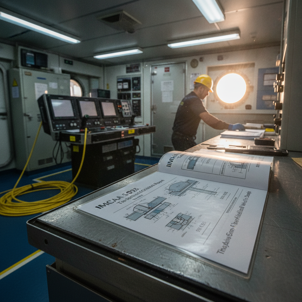
IMCA S 026, unpacked: what an out-of-straightness survey actually requires
IMCA S 026 out-of-straightness survey guidance, unpacked: the checks, error budget, deliverables and QC it actually specifies for rigid subsea pipelines – and where it leaves the numbers to your project procedures.
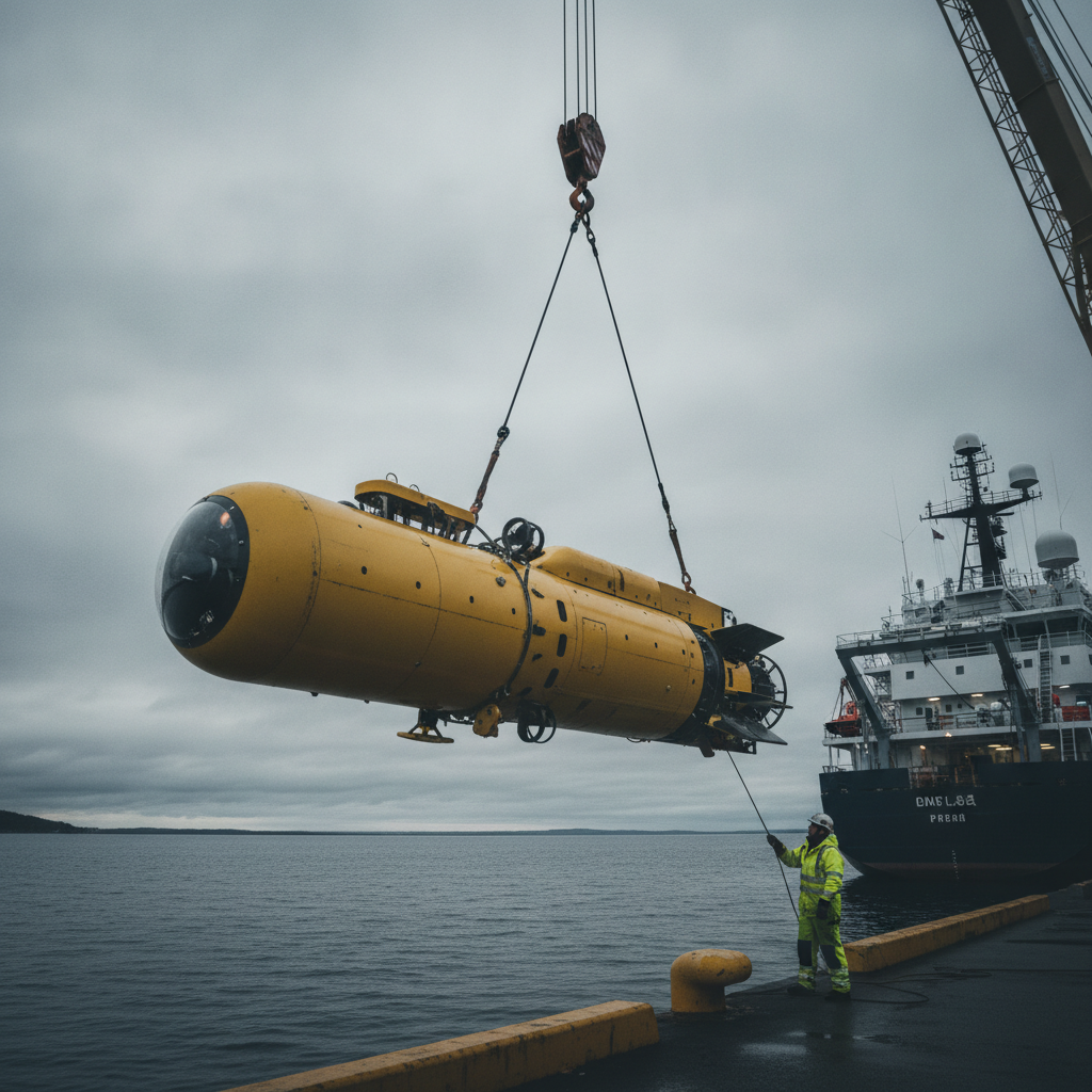
Buy the AUV or the capability? The HUGIN Superior question
Norway's HUGIN Superior brings deep-sea AUV mapping in-house. We unpack the navigation, bathymetry and assurance decisions owners face at 6,000 m and high latitude.
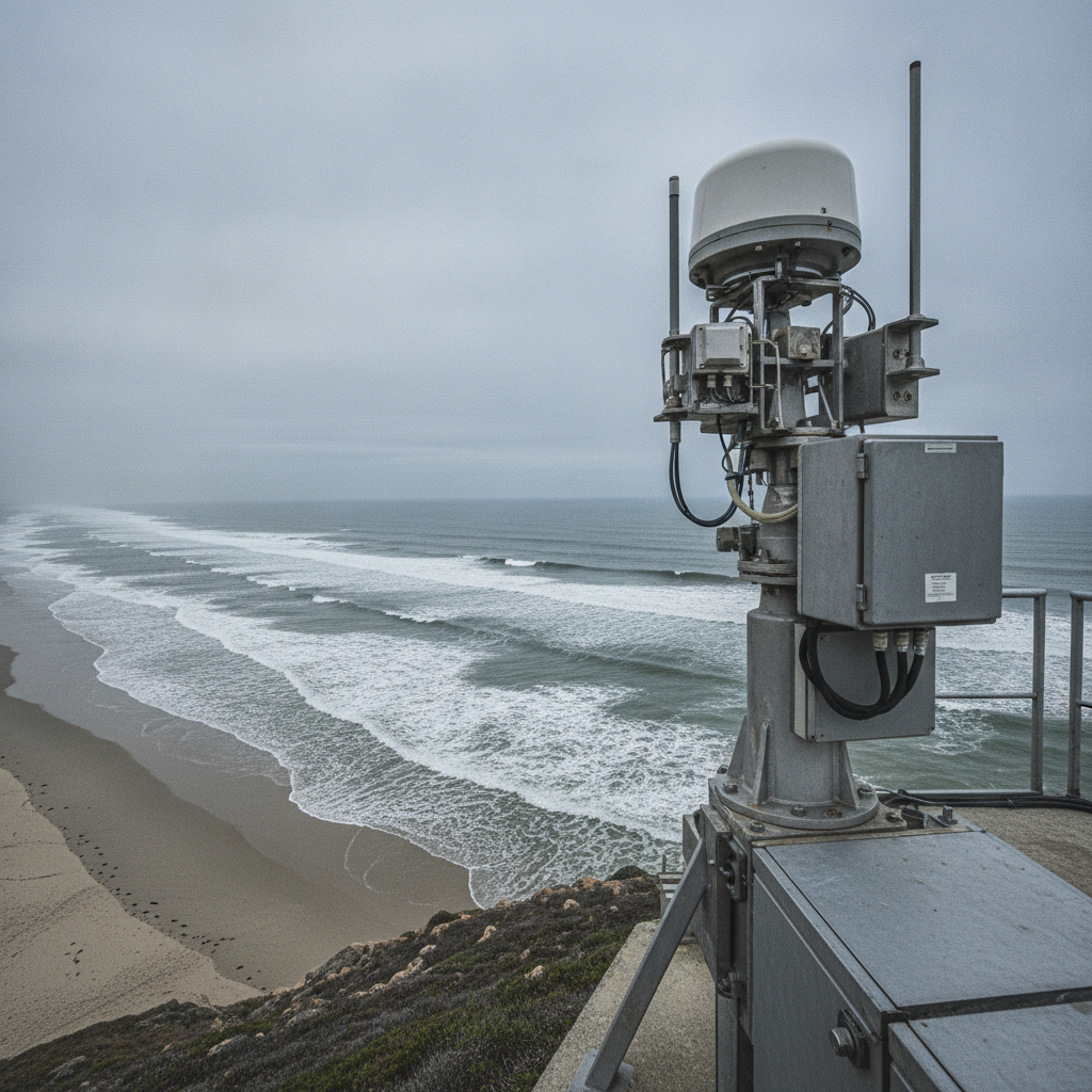
Radar-derived bathymetry: where wave inversion sits beside multibeam
How X-band radar sea-state inversion estimates depth, where it meets and misses IHO S-44, and how to blend it with multibeam for nearshore monitoring.
Offshore Geomatics Foundation Certificate · October 2026
Turn reading into certified competence
You have just read what a standard actually requires – and where it stops. The Foundation Certificate exists to prove you can work with that distinction.
Early-access list gets 40% off at launch. No spam – the waitlist is only ever used for the certificate. What the certificate covers →