Executive Summary
Recent research shows multibeam echosounder water column data can move beyond detecting gas plumes to estimating gas flow, offering a scalable alternative to ROV and lander surveys. The acoustic estimate is a chain of conversions, each with real uncertainty, and without site-referenced calibration it is a relative index rather than an absolute flux. This brief unpacks the physics, the calibration limits, the absence of any water column standard, and sets out concrete criteria for choosing between MBES and dedicated in-situ measurement.
On this page5 sections
What the recent research puts on the table
Recent research makes a straightforward but consequential argument: multibeam echosounder (MBES) water column data, long treated as a by-product of bathymetric acquisition, carries quantitative information about how much gas is leaving the seabed. The work – presented with data courtesy of NIOZ and TNO – pushes the discussion past detection, which the hydrographic community already handles well, toward the remote estimation of gas flow.
The framing matters because gas release takes many forms: natural methane seepage, leakage from abandoned wells, and losses from subsea infrastructure such as pipelines, with future carbon storage sites now added to the list. MBES that record the water column are proven for finding bubble streams. They give wide area coverage and sit on most survey vessels, which is exactly why they attract interest for the harder task of quantification. The alternative – direct in-situ measurement with ROVs or seabed landers – is accurate but expensive, operationally heavy, and does not scale when there are dozens or hundreds of individual streams to assess.
Historically, the interpretation of acoustic plumes (the vertical columns of enhanced backscatter that rising bubbles produce) has been qualitative: counting streams, describing their height and shape. The step the research advances is turning that backscatter into a gas flow rate, with the stated caveats that the estimates are coarse and demand genuine skill in acoustic calibration. That is the honest starting point. The rest of this analysis is about where the resulting number can be trusted and where it cannot.
What the acoustics actually measure
A gas bubble is an efficient acoustic scatterer for two reasons: the impedance contrast between gas and water is large, and bubbles resonate. The Minnaert resonance frequency scales inversely with bubble radius – a millimetre-radius bubble resonates at a few kilohertz near the surface, and that frequency rises with depth as pressure increases. Working MBES bands, roughly 12 to 500 kHz depending on operating depth, generally sit well above resonance for the bubble sizes that dominate most seeps. Above resonance, the backscattering cross-section of a bubble tends toward its geometric cross-section, scaling with the square of the radius.
That detail is the whole problem in miniature. The system measures a volume backscattering strength that sums the backscatter cross-sections of every bubble in the insonified volume – a quantity proportional to the sum of radius-squared. What we actually want is the gas volume flux, which depends on void fraction (the sum of radius-cubed) multiplied by bubble rise velocity and the cross-sectional area of the plume. Converting between the two requires the bubble size distribution. A single-frequency MBES does not resolve that distribution; it must be assumed, measured optically, or constrained with multi-frequency acoustics.
Rise velocity introduces a second dependency, because it is also a function of bubble size and of whether bubble surfaces are clean or coated with surfactants – typically tens of centimetres per second for millimetre bubbles, but not a fixed constant. Bubbles do not keep their identity as they ascend either. Gas expands as pressure drops, methane dissolves into undersaturated seawater, and gas exchange alters composition. Seabed flux, flux at mid-water, and any flux that survives to the sea surface are three different numbers, and the difference between them grows with water depth.
So the acoustic estimate is a chain of conversions: measured backscatter, then an assumed size distribution, then void fraction, then rise velocity, then flux at the measurement depth, and optionally seabed or sea-surface flux. Each link carries its own uncertainty. Every one of them has to be defensible for the final figure to mean anything to a client or a regulator.
Calibration is the part most teams underestimate
Scientific split-beam echosounders of the EK60 and EK80 class are routinely calibrated with tungsten-carbide standard spheres, so that absolute volume backscattering strength is traceable. MBES are a harder case for water column work. The beam pattern varies across a wide swath, sensitivity changes from nadir to the outer beams, time-varying gain has to apply the correct spreading law for a diffuse volume target rather than a point target on the seabed, and near-field geometry complicates the region close to the transducer. Most MBES are optimised and calibrated for seabed detection, not for absolute backscatter from bubbles suspended in mid-water.
Without a site-referenced calibration, the number an MBES produces is a relative index, not an absolute flux. That is not a fatal weakness – a well-behaved relative index is exactly what triage needs – but it has to be stated plainly in the deliverable rather than dressed up as an emission figure.
The governing gap here is the absence of an agreed standard. IHO S-44 sets bathymetric accuracy standards and is silent on water column backscatter and on flux. The backscatter guidance the marine acoustics community has produced addresses seafloor backscatter for habitat and sediment classification, not gas plumes rising through the water. There is, at present, no equivalent acceptance framework that tells a survey manager what uncertainty budget, calibration regime, or reporting format a quantified seepage estimate must meet. Until one exists, the burden falls on the contractor to define and document the method, which is uncomfortable when the output feeds regulatory or financial decisions.
Where MBES quantification earns its place
The strongest case for acoustic quantification is prioritisation across a large area. When a survey identifies many bubble streams, deploying an ROV to each one is neither affordable nor operationally sensible. An MBES pass that ranks streams by relative flux lets you focus the expensive in-situ effort on the handful of sites that dominate the total, which is usually a small fraction of the count. For screening leaks at pipelines, wells, and prospective carbon storage sites, a relative index that flags where something changed is often the decision the operator actually needs.
Temporal monitoring is the second strong case. If the same MBES, on the same vessel, with the same settings, repeats a line over months or years, systematic errors cancel and the trend in backscatter becomes a defensible proxy for whether a seep is growing, stable, or shrinking – even where the absolute flux stays uncertain. This is the same logic that governs long-term baseline environmental monitoring in other domains, where regulatory appetite for precise absolute numbers frequently outruns what the sensors can honestly deliver, a tension we have examined in the context of ADCP-based monitoring for deep-sea mining environmental assessments.
The practical payoff is real: faster, more flexible surveys from smaller vessels at lower cost than an ROV or lander campaign. The condition attached is equally real. The acoustic method earns its place when relative comparison and coverage matter more than a traceable absolute number.
Where dedicated in-situ methods still win – and how to decide
Direct measurement stays the reference where the absolute number is the product. Emissions accounting under measurement-based reporting expectations, and monitoring, measurement and verification for offshore CO2 storage under DNV recommended practice and ISO 27914, both demand quantified flux with a stated uncertainty. An uncalibrated acoustic index does not meet that bar on its own. Dense plumes present a second limit: near a vigorous vent the void fraction is high enough that multiple scattering and attenuation distort the backscatter, and the acoustic estimate saturates precisely where the flux is largest.
A point worth making to anyone reaching for the phrase “gas sensor”: dissolved-methane chemical sensors, whether membrane-type or laser-based, measure concentration in the water, not flux from the seabed. They answer a different question. They are valuable for confirming that methane is present and for mapping dissolved plumes, but they do not substitute for either acoustics or direct volumetric capture when the deliverable is a flow rate.
On that basis, we would build a seepage assessment around the following:
- Anchor the acoustics to ground truth. Carry ROV bubble-capture or a calibrated seabed lander on a representative subset of streams, and derive a site-specific regression between integrated backscatter and measured flux. Report acoustic-only streams as order-of-magnitude estimates with explicit bounds until that regression exists.
- Constrain the bubble size distribution rather than assuming it. Use multi-frequency acoustics where available, or optical bubble sizing from the ROV, because the radius-squared-to-radius-cubed conversion is the single largest source of error in the chain.
- Calibrate the system for water column work. Where absolute figures are required, run a split-beam echosounder alongside the MBES as a calibrated reference, and record the sound-speed profile, temperature and salinity that the flux conversion depends on.
- Fix the survey geometry. Repeat lines with identical settings for temporal work, and account for tidal and current advection that bends plumes off vertical between the seabed source and the sensed depth layer.
- State the reference depth. Make clear whether a reported flux is at the sensed depth, back-calculated to the seabed, or estimated at the sea surface. Conflating these is the most common way seepage numbers are misread.
- Manage the data volume from the outset. Water column recording generates far more data than bathymetry; retain the raw water column, not just derived plumes, and hold it in a structured survey data model so the estimates remain auditable. The direction set by the latest revision of the IOGP seabed survey data model is a sensible reference point for how that structuring should look.
The judgement, then, is not MBES versus in-situ. It is a two-tier design: acoustics for coverage, ranking and trend across the whole field, and dedicated measurement on the streams that matter and on the subset needed to calibrate the rest. Treat the MBES output as an absolute emission figure without that calibration and the method will not survive scrutiny. Treat it as a scalable, relative, well-documented index tied to ground truth, and it does exactly the job the research claims for it.
Based on: MBES as a practical tool for seepage impact assessments
Published by
Hydrographic Methods Committee
Bathymetry, Multibeam & Seabed Mapping
An independent review committee focused on hydrographic survey methodology, IHO standards interpretation, and seabed mapping best practices for offshore and coastal projects.
Read next
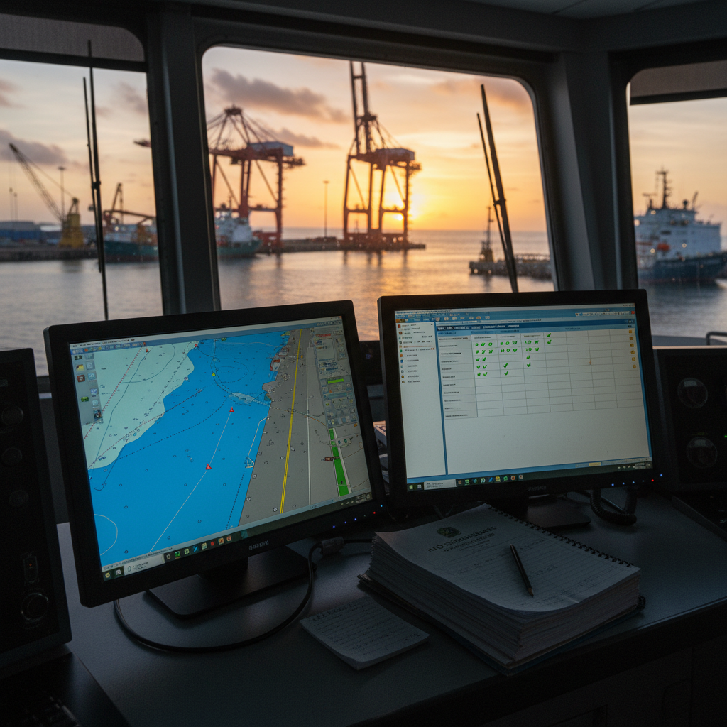
Brazil's first S-101 ENC: what survey contractors should plan for
Brazil's first S-101 ENC at Suape begins its dual-fuel transition. What survey contractors in Brazilian waters should plan for in deliverables and QC.
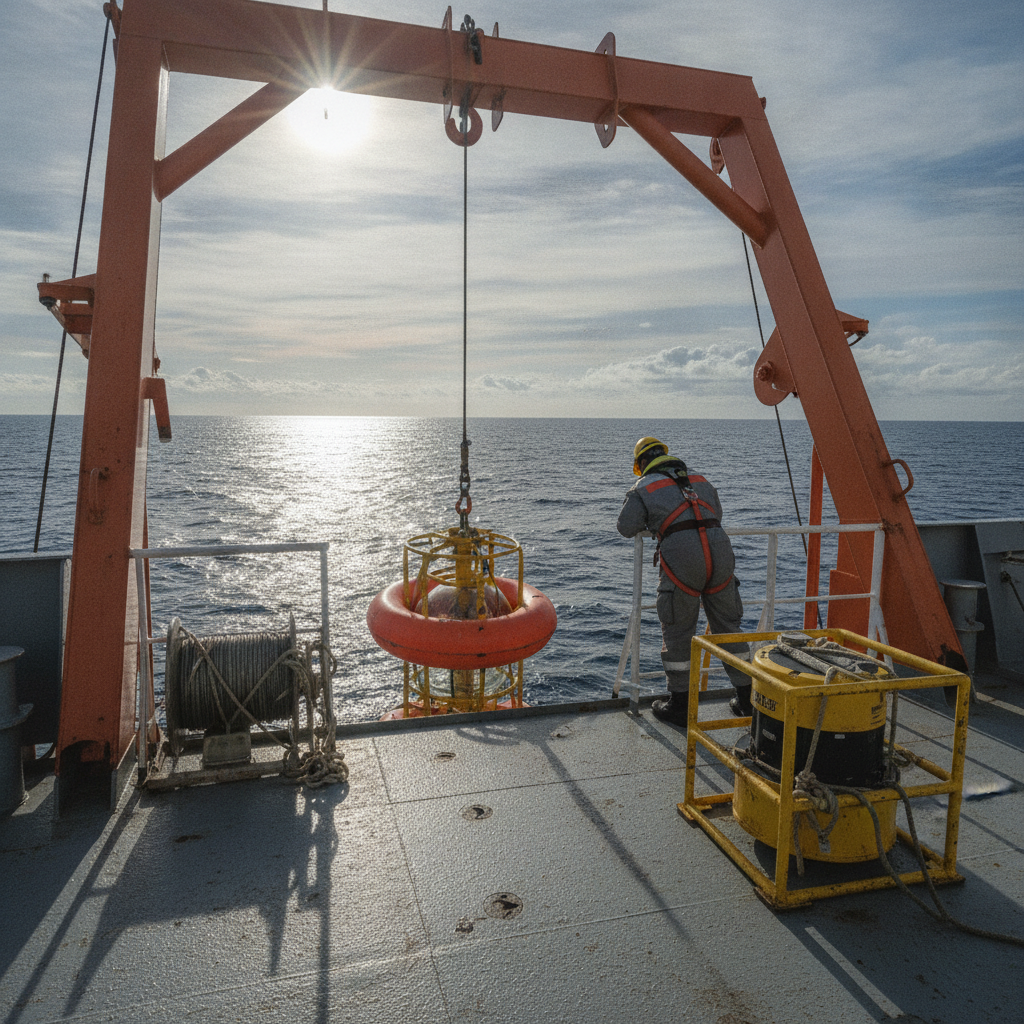
Deep-sea mining EIAs: ADCP deployment reality vs regulatory demand
Deep-sea mining EIA baseline monitoring with ADCPs: what ISA rules require for currents and sediment plumes, and where survey managers under-scope.

IMCA S 026, unpacked: what an out-of-straightness survey actually requires
IMCA S 026 out-of-straightness survey guidance, unpacked: the checks, error budget, deliverables and QC it actually specifies for rigid subsea pipelines – and where it leaves the numbers to your project procedures.
Offshore Geomatics Foundation Certificate · October 2026
Turn reading into certified competence
You have just read what a standard actually requires – and where it stops. The Foundation Certificate exists to prove you can work with that distinction.
Early-access list gets 40% off at launch. No spam – the waitlist is only ever used for the certificate. What the certificate covers →